Predicting User Persona Segments from Ride-Hailing Behaviour
Members
01Nguyễn Giao Chi
02Trần Anh Minh
03Huỳnh Ngọc Tấn Thuận
04Huỳnh Trọng Nghĩa
05Nguyễn Quốc Khánh
06Ngô Quốc Đạt
II. Problem and objectives
Background
Ride-hailing platforms record millions of GPS-based trips, but know little about who their riders are. Pick-up/drop-off locations, POIs and time of day carry strong hints about a rider's daily routine. This project uses 4.87M trips from 47,322 riders in Ho Chi Minh City and Hanoi (Jan–Aug 2026).
Motivation
Knowing a rider's segment enables better offer design, targeted promotions and service planning without asking riders for personal information. Behaviour-based tags are cheaper and more scalable than surveys, provided they are accurate and used responsibly.
Research question(s)
Can ride behaviour alone classify a rider as Office WorkerParentor University Student?
Which behavioural signals (locations, POIs, time windows) best separate the three segments?
Which model (KNN, Decision Tree, Random Forest, Gradient Boosting) performs best, measured by macro-F1?
Define the scope: Use xMap mobility data (GPS pings) in Ho Chi Minh City and Hanoi from 01/01 to 28/02/2026, including the Tết period. Prioritise a set of devices that remain consistently active across both months.
Detect stay points: Cluster pings into stay points, i.e. places where a device remains long enough. From these, infer home (night-time location) and work/study place (daytime location on weekdays).
Assign segments using POIs: Match stay points against xMap POIs:
University Student regularly present at a university or college.
Parent short visits to a kindergarten or primary school during morning and afternoon drop-off/pick-up hours.
Office Worker stays at an office building throughout business hours on weekdays.
Each user belongs to exactly one segment.
Build trips: Each movement between two consecutive stay points counts as one trip. Each trip records origin and destination, start and end time, distance, travel time, city, and the nearest address or POI at pick-up/drop-off.
Enrich the data: Estimate the vehicle type (motorbike or car) from speed and distance. Use road traffic data to add speed, congestion level and ETA by time window. Where possible, flag trips that are likely ride-hailing trips.
Deliver: One row per trip, anonymised IDs, exported as CSV or Parquet split by month.
Required fields
User ID (anonymised), segment, city, date, departure/arrival time, origin/destination coordinates, pick-up and drop-off POI/address, distance, travel time, estimated vehicle type.
Accuracy expectations
Accuracy is only needed at the level of trends and distributions, not individual trips. Prioritise coverage, a sufficiently large panel and stability over eight months.
Retains riders and handles unavailable measurements without learning from test data.
Không điền tọa độ hoặc thời gian giả. Tọa độ không hợp lệ không khớp POI; timestamp thiếu không tham gia điều kiện giờ/ngày hoặc tính thời gian ở lại.
Latitude ngoài [−90, 90], longitude ngoài [−180, 180], giá vé/discount âm, surge không dương và giá trị số không hữu hạn được coi là missing. Không xóa chuyến vì các lỗi này.
Thiếu địa chỉ được biểu diễn bằng chuỗi rỗng để kiểm tra regex. Điều kiện POI/địa chỉ không khớp đóng góp 0 vào tử số; mẫu số tỷ lệ vẫn là toàn bộ chuyến của rider. Không khớp POI không khẳng định đó là nhà.
Ở cấp feature: thay ±inf, giá trị ngoài miền hợp lệ và o_lai_median_gio = -1 bằng missing. Điền median của tập train; với hai cờ nhị phân dùng mode của train, hòa chọn 0.
Nếu toàn bộ giá trị của một feature trên train đều thiếu, dùng 0 làm fallback và ghi lại trong state.
Giữ mọi rider có ID hợp lệ. Thiếu rider_id thì dừng với lỗi; không gộp những người thiếu ID thành một người giả.
Nếu một rider có nhiều user_tag khác nhau, dừng để xử lý nhãn nguồn. Nếu chỉ thiếu nhãn, đưa rider vào nhóm unlabeled, không dùng để fit hay đánh giá.
Outliers
Validity checks and train-fitted P1–P99 winsorization on six features.
Limits extreme values while preserving rows, bounded shares and rare binary signals.
Ngưỡng dưới/trên là P1/P99 của các quan sát hợp lệ thuộc train, trước imputation. Cùng ngưỡng đó được dùng cho train, test và inference.
Giá trị vượt ngưỡng được đưa về ngưỡng; không loại dòng. Nếu hai ngưỡng bằng nhau, bỏ clipping ở cột đó.
54 feature tỷ lệ và 2 cờ nhị phân không bị winsorize. Ngưỡng cấu hình qua --clip-lower và --clip-upper.
Encoding
Binary/share predictors; separate label encoding for user_tag.
Converts categories to numeric inputs; keeps IDs and target labels outside X.
Các loại POI/service được chuyển thành feature chỉ báo hoặc tỷ lệ chuyến, không dùng mã số nguyên tùy ý. Bộ X đã có 62 feature dạng số nên không cần one-hot lại.
rider_id chỉ là khóa liên kết; user_tag là biến mục tiêu. Cả hai đều bị loại khỏi X.
LabelEncoder học các nhãn trong train: Office Worker → 0Parent → 1University Student → 2. Mã là nhãn danh nghĩa, không biểu thị thứ bậc.
Nhãn thiếu/nhãn mới ở inference có mã −1. Nhãn test chưa từng có trong train sẽ gây lỗi thay vì bị gán vào lớp khác.
Scaling
Train-fitted z-scores for 60 features; two binary flags unchanged.
Makes numeric scales comparable and applies consistent transformations to held-out data.
z = (x − mean_train) / std_train
Mean/std được tính sau imputation và clipping, chỉ trên train; std dùng ddof=0. Cột không có phương sai dùng hệ số chia bằng 1.
Hai cờ neo_la_truong_pt, neo_la_dai_hoc giữ 0/1.
--scale standard mặc định · --scale robust median/IQR · --scale none giữ thang đo sau imputation/clipping.
Feature engineering
62 rider-level POI, time, address, mobility, seasonal and spending features.
Summarizes repeated travel behavior and trip context for rider classification.
Gộp pickup/drop, làm tròn 5 chữ số; lưới 0,005°; nhân POI sang 9 ô; tính haversine và lấy POI gần nhất trong 25 m.
Đổi timestamp UTC sang UTC+7 trước khi tính giờ/ngày/tuần/tháng. Khoảng giờ gồm cả hai đầu (06–09h là 06:00 đến 09:59:59).
Giữ tất cả chuyến, không tự lọc trạng thái và không loại chuyến trùng. Không dùng user_tag để tính feature hành vi.
Home là pickup phổ biến nhất 06–09h; anchor là drop phổ biến nhất ngày thường 06–18h khác home (ô làm tròn 3 chữ số).
addr_ngo_hem, addr_nha_den_truong, addr_nha_den_office vẫn giống nhau theo cấu hình regex mặc định.
Matching POI ≤25 m và “POI null” là proxy; không phải kết luận đã xác minh về nơi ở hoặc nghề nghiệp.
Output · Lean data dictionary lean.csv · 1 row per rider · 64 columns
Share of trips whose pickup / drop address text contains a keyword (đại học, THPT, tòa nhà, chung cư, ngõ, ký túc xá, bệnh viện…)
Home ↔ school / office flows 9nha_den_truongnha_den_officetu_truong_vedr_edu_ampu_edu_pmdr_edu_pmaddr_nha_den_truongaddr_nha_den_officeaddr_truong_ve_nha
Numeric
Share 0–1
Trip direction patterns: home→school, school→home, home→office, plus school trips in morning (06–09h) and afternoon (15–18h)
sh_* time of day 6sh_am_peaksh_wd_vao_cash_wd_truash_wd_16hsh_wd_toish_night
Numeric
Share 0–1
Share of trips booked in specific time windows (morning peak, lunch, 16h, evening, night), weekday vs all days
Anchor point 5neo_la_truong_ptneo_la_dai_hocsh_toi_diem_neosh_nha_diem_neotuan_co_diem_neo
Binary / Numeric
0/1, Share
Rider’s most frequent destination cell: whether it is a school or university, and how often trips / weeks touch it
Service mix 3sh_carsh_foodsh_deli_wd_gio_hc
Numeric
Share 0–1
Share of trips by service: car, food, delivery during office hours
Seasonality 2tet_vs_hoc_kytruong_he_vs_hoc_ky
Numeric
Ratio
Trip volume in Tết and summer break vs regular school months
Active days, pickup & driver diversity, discount rate, average surge, median dwell time between trips
V. Exploratory data analysis
All EDA uses the 80% Learning set only (37,858 riders), so the Test set stays unseen until final evaluation.
Office WorkerParentUniversity Student
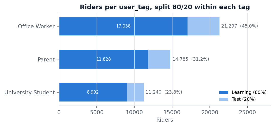
Chart 1 · Class balance and split
Insight: The classes are imbalanced (45 / 31 / 24%). Always guessing "Office Worker" already reaches 45% accuracy, so every split is stratified and models are selected by macro-F1 rather than accuracy.
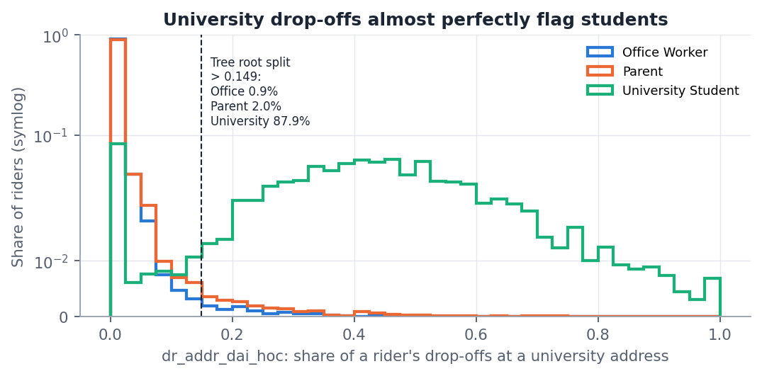
Chart 2 · University drop-off signal
Insight: 87.9% of students drop off at a university address on more than 14.9% of their trips, against 0.9% of office workers and 2.0% of parents. This one feature almost isolates the student class.
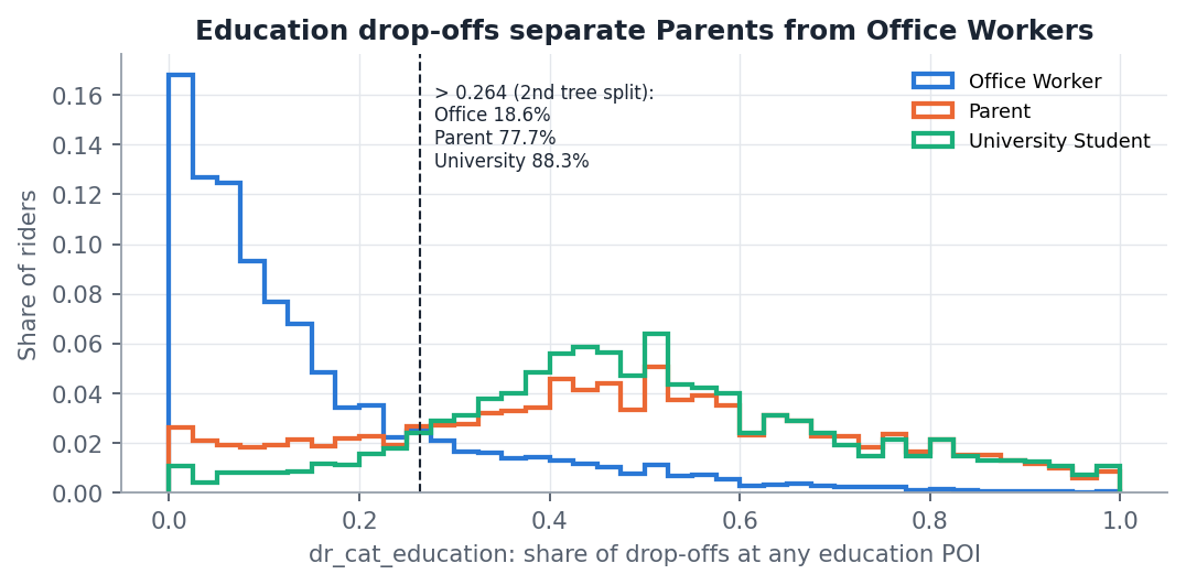
Chart 3 · Education drop-offs
Insight: 77.7% of parents end more than 26.4% of their trips at an education POI, against 18.6% of office workers. Students score high too, so this feature splits Parent from Office only after students are removed by Chart 2's signal.
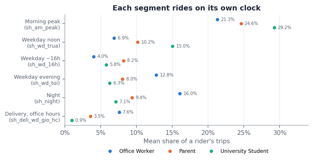
Chart 4 · Time-of-day fingerprint
Insight: Each segment keeps its own schedule:
OfficeOffice workers ride more at night (16.0%) and on weekday evenings (12.8%), and order more deliveries in office hours.
ParentParents peak around the 16h school pick-up (8.2% vs 4.0% for office workers).
StudentStudents ride most at noon (15.0%).
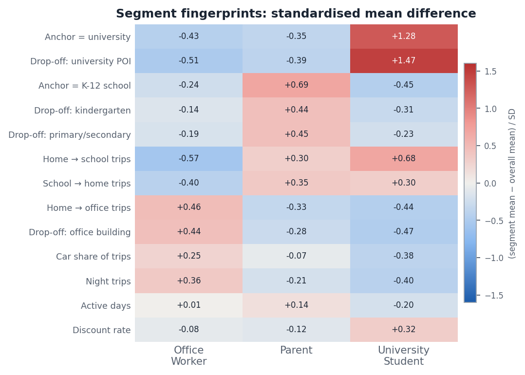
Chart 5 · Segment fingerprints
Insight: Each segment has a distinct anchor:
StudentStudents: +1.47 SD on university drop-offs.
ParentParents: +0.69 SD on a K-12 school anchor.
OfficeOffice workers: +0.46 SD on home → office trips, plus more car and night trips.
The features are behaviourally meaningful, not noise.
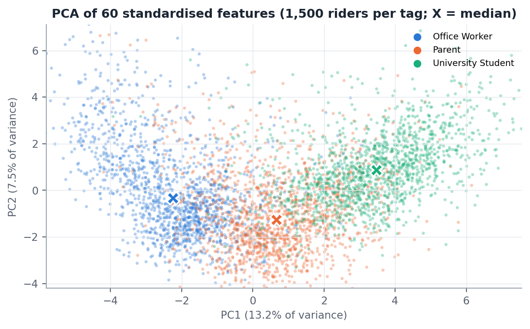
Chart 6 (optional) · Class separability
Insight: Students form their own cluster, while Office and Parent overlap in the middle. The first two components explain only 20.8% of variance, so non-linear models are needed. The overlap anticipates where most prediction errors fall.
We train four classifiers to guess each rider's user_tag from 60 behaviour features. To make the contest fair, all four use the same riders, the same features, the same practice rounds and the same final exam. Only the model and the settings it tries are different.
The workflow in five steps identical in all four scripts
1Split the riders
Within each tag, shuffle riders (seed 42). 80% go to Learning, 20% to Test.
Learning37,858
Test9,464
Learning only
2Clean features
Drop columns that never change or copy another column.
Features 62 → 60
Learning only
3Practice and tune
Try many settings. Score each one with 5-fold cross-validation.
Score = macro-F1
Learning only
4Retrain the winner
Fit the best setting again on all Learning riders.
One final model each
Test 9,464 riders stay locked. Nothing in steps 2–4 looks at them.
5Final exam, once
Predict the locked Test riders one time and compute the scores in section VII.
No retuning afterwards
Step 1 · Each tag is split on its own
Office Worker21,297 · test 4,259
17,038
Parent14,785 · test 2,957
11,828
University Student11,240 · test 2,248
8,992
Learning 80%Test 20%
So both sets keep the same mix of 45% Office, 31% Parent, 24% Student, and no rider appears in both.
Step 3 · 5-fold cross-validation = five practice exams
Round 1
Round 2
Round 3
Round 4
Round 5
Train on ≈ 30,286Score on ≈ 7,572
Each setting is trained 5 times, each time scored on riders it did not see. Its CV score is the average of the 5. All models use the same 5 folds.
The four models from one simple model to teams of trees
Model 1 · Instance-based
K-Nearest Neighbours
CV macro-F10.884
The 11 most similar riders vote, and closer riders count more. Here: 7 Office, 3 Parent, 1 Student, so the answer is Office Worker.
Ask the neighbours. To tag a new rider, find the 11 riders in the Learning set whose behaviour is most similar and take their weighted vote. The model learns nothing in advance; it compares at prediction time, so features must first be put on the same scale.
SettingTriedChosen
Neighbours K30 values, 1 … 15111
Distancestraight-line or ManhattanManhattan
Voteequal, or closer counts morecloser counts more
ScalingStandard or Min-MaxStandard
48 settings triedpicked by 5-fold CV
How it predicts. No parameters are learned; the model stores all scaled learning riders and measures distance at prediction time.
Coarse search for K over 30 values with the default distance (Euclidean, equal votes).
Fine search around the best K (K−2, K, K+2) × distance × vote weights × scaler: 18 configurations.
Refit the best pipeline; the scaler is refit inside every CV fold, so validation riders never shape the scaling.
Hyperparameter
Searched
Selected
n_neighbors
{1, 3, …, 51, 61, 75, 101, 151}, then K ± 2
11
p (distance)
2 = Euclidean, 1 = Manhattan
1 · Manhattan
weights
uniform, distance
distance
scaler
StandardScaler, MinMaxScaler (MinMax tried with Euclidean only)
Standard
Muốn đoán nhóm của một rider mới, KNN tìm 11 rider giống nhất trong tập Learning rồi cho họ “bỏ phiếu”. Người càng giống thì phiếu càng nặng (trọng số 1/khoảng cách).
“Giống” được đo bằng tổng chênh lệch tuyệt đối của 60 feature (Manhattan). Phải chuẩn hoá trước, nếu không feature có thang đo lớn như active_days sẽ lấn át các tỷ lệ 0–1.
KNN không học tham số nào: nó nhớ toàn bộ 37,858 rider và tính khoảng cách tới tất cả khi dự đoán (algorithm="brute"). Vì vậy đây là mô hình dự đoán chậm nhất.
Model 2 · Single tree
Decision Tree
CV macro-F10.871
Simplified view of the first two questions. The real tree asks up to 12 questions in a row and ends in 103 leaves.
A flowchart of yes/no questions. The tree picks the question that best separates the three tags, then repeats inside each branch. A tree that grows too far memorises the riders it was trained on, so it is cut back (pruned) until the cross-validation score is highest.
SettingTriedChosen
Split ruleGini or entropyGini
How to prunestop early (168 combos) or grow, then cut (26 levels)grow, then cut
Cut strength α0 to 0.010.000237
Final size12 levels, 103 leaves
194 settings triedpicked by 5-fold CV
How it learns. At each node, try every feature and threshold, and keep the split that makes the two child groups purest. Then prune back the branches that do not pay for their size.
Gini(t) = 1 − Σc pc² (entropy also tried) best split = max [ I(parent) − Σ (nchild/n)·I(child) ] pruning: Rα(T) = R(T) + α·|leaves(T)|
Path A, pre-pruning: stop growth early with max_depth × min_samples_leaf (168 configurations).
Path B, post-pruning: grow the full tree with Path A's criterion, then cut back with cost-complexity α (26 values).
Keep the path with the higher CV macro-F1. Path B won.
Hyperparameter
Searched
Selected
criterion
gini, entropy
gini
max_depth
2–8, 10, 12, 15, 20, None (Path A)
not limited
min_samples_leaf
1, 5, 10, 20, 50, 100, 200 (Path A)
1 (default)
ccp_alpha
0 and 25 log-spaced values 10⁻⁵…10⁻² (Path B)
2.37 × 10⁻⁴
Cây hỏi lần lượt các câu có/không trên từng feature. Mỗi câu được chọn sao cho hai nhóm con “thuần” nhất, tức mỗi nhóm chủ yếu chỉ có một loại rider (Gini giảm nhiều nhất).
Nếu để cây mọc tự do, nó sẽ học thuộc tập Learning (overfit). Code thử hai cách tỉa: tỉa trước (giới hạn độ sâu, số rider tối thiểu ở lá) và tỉa sau (cho mọc hết rồi cắt các nhánh có lợi ích nhỏ hơn chi phí α cho mỗi lá). Tỉa sau thắng.
Cây chỉ so sánh với ngưỡng nên không cần chuẩn hoá dữ liệu.
Model 3 · Many trees in parallel
Random Forest
CV macro-F10.899
Each tree learns from a different random resample of riders and sees only 19 of the 60 features at each question. The forest averages their answers.
Wisdom of the crowd. Grow 500 different trees, each from a random resample of riders and a random subset of features, then average their answers. Each tree makes different mistakes, so averaging cancels many of them.
SettingTriedChosen
Number of treesfixed500
Features per question7, 5 or 19 of 6019
Min riders per leaf1, 3 or 51
9 settings triedpicked by out-of-bag score
How it learns. Many deep, de-correlated trees each overfit in a different way; averaging cancels much of that variance.
P̂(c | x) = (1/500) Σb P̂b(c | x), ŷ = argmaxc P̂(c | x) each rider is out-of-bag for ≈ (1 − 1/n)n ≈ 36.8% of trees
Fit 9 forests (3 max_features × 3 min_samples_leaf), 500 trees each.
Score each with OOB macro-F1: every rider is predicted only by trees that never saw it, so no separate validation set is needed. Best OOB = 0.899.
Check with 5-fold CV for a score comparable to the other models (0.899), then refit on all Learning riders.
Hyperparameter
Searched
Selected
n_estimators
fixed
500
max_features
√m = 7, log₂m = 5, 0.33·m = 19 (m = 60)
0.33 · 19
min_samples_leaf
1, 3, 5
1
Trồng 500 cây. Mỗi cây học trên một mẫu bootstrap (rút có hoàn lại 37,858 rider) và ở mỗi nút chỉ được xét ngẫu nhiên 19/60 feature. Nhờ vậy các cây khác nhau, và khi lấy trung bình xác suất của 500 cây, lỗi riêng của từng cây phần lớn triệt tiêu.
Khoảng 37% rider không nằm trong mẫu của một cây bất kỳ (out-of-bag). Dùng các cây “chưa thấy” rider đó để chấm điểm thì có ngay một bộ validation miễn phí. Code chọn tham số theo điểm OOB này, còn 5-fold CV chỉ để so sánh công bằng với ba mô hình kia.
Model 4 · Many trees in sequence
Gradient Boosting Best
CV macro-F10.904
Schematic. Training keeps improving, but the score on held-out riders stops improving. Training stops 30 rounds after the best point. Final model: 485 rounds.
Learn from mistakes, one small step at a time. Trees are added one after another. Each new small tree focuses on the riders the model still gets wrong and adds only a small correction. Training stops automatically when held-out riders stop improving.
SettingTriedChosen
Learning rate0.03, 0.1 or 0.30.03
Leaves per tree15, 31 or 6315
L2 penalty0 or 10
Roundsauto-stop, max 2,000485
18 settings triedpicked by 5-fold CV + auto-stop
How it learns. Start from the class priors. Each round grows one small tree per class (3 per round) on the residual y − p, which is the negative gradient of the multinomial log-loss, and adds it with a small step η.
Fm(x) = Fm−1(x) + η·hm(x), p = softmax(F) ric = yic − pc(xi) (leaf values: Newton step with L2 penalty λ) features are binned to ≤ 255 values so split search is fast
Grid search 3 learning rates × 3 tree sizes × 2 L2 penalties = 18 configurations under 5-fold CV.
Inside every fit, up to 2,000 rounds, with early stopping on 10% of that fit's own training data. The CV validation fold is not used for stopping.
Refit the best configuration on the Learning set (90% grows trees, 10% decides when to stop). It stopped at 485 rounds, i.e. 485 × 3 = 1,455 trees.
Hyperparameter
Searched
Selected
learning_rate (η)
0.03, 0.1, 0.3
0.03
max_leaf_nodes
15, 31, 63
15
l2_regularization
0, 1
0
rounds (n_iter_)
early stopping: patience 30, max 2,000
485
Random Forest trồng cây song song; boosting trồng cây nối tiếp. Mỗi vòng thêm 3 cây nhỏ (≤ 15 lá, mỗi lớp một cây) chuyên sửa phần mà các vòng trước còn đoán sai, rồi chỉ cộng 3% đóng góp của chúng (learning rate 0.03).
Học chậm thì cần nhiều vòng, nhưng quá nhiều vòng sẽ overfit. Vì vậy early stopping giữ riêng 10% dữ liệu huấn luyện, theo dõi loss trên phần đó và dừng khi 30 vòng liền không cải thiện. Mô hình cuối dừng ở vòng 485.
Chữ “Hist” nghĩa là mỗi feature được gom vào tối đa 255 nhóm giá trị trước khi tìm ngưỡng chia, giúp chạy nhanh trên 37,858 rider.
How the models are scored on the 9,464 Test riders
Metric
In plain words
Used for
Macro-F1
F1 for each tag, then the average. Small tags (Student, Parent) count as much as the 45% Office majority, which is why this is the main score.
Choosing & ranking
95% CI of macro-F1
Resample the Test riders 1,000 times. The range shows how much the score could move with a different Test sample.
How well the predicted probabilities rank the true tag first. 0.5 = coin flip, 1 = perfect.
Reporting
RMSE* and R²*
How close the predicted probabilities are to the truth (1 for the true tag, 0 for the others). R² = 0 means no better than guessing the class shares.
Supporting
*RMSE and R² are regression metrics, so here they are applied to probabilities.
F1c = 2·Precisionc·Recallc / (Precisionc + Recallc); macro-F1 = (F1Office + F1Parent + F1Student) / 3 RMSE = √[ (1/3n) Σi Σc (yic − p̂ic)² ]; R² = 1 − Σ(y − p̂)² / Σ(y − π)², π = Learning class shares (0.45 / 0.31 / 0.24) ROC-AUC = mean over tags of AUC(tag vs rest); 95% CI = 2.5th–97.5th percentile of 1,000 bootstrap macro-F1 values. Balanced accuracy (mean recall) is also saved in metrics.json.
VII. Results and evaluation
Best modelGradient Boostingbest on every metric
Test macro-F10.90495% CI 0.898–0.910 · baseline 0.207
Accuracy90.0%baseline 45.0%
ROC-AUC0.9780.5 = coin flip
Model comparison Test set, 9,464 riders · ranked by Test macro-F1
Model
Accuracy
F1 (macro)
F1 95% CI
CV F1
RMSE*
R²*
ROC-AUC
Rank
Gradient Boosting
0.900
0.904
0.898–0.910
0.904
0.221
0.772
0.978
1
Random Forest
0.891
0.895
0.888–0.900
0.899
0.233
0.747
0.974
2
KNN
0.882
0.884
0.877–0.891
0.884
0.243
0.725
0.963
3
Decision Tree
0.862
0.867
0.861–0.874
0.871
0.264
0.676
0.955
4
Baseline (always “Office Worker”)
0.450
0.207
–
–
0.463
0.000
0.500
–
*Classification task: RMSE and R² are computed on predicted probabilities vs one-hot labels (see VI). Lower RMSE and higher values elsewhere are better.
RMSE = √mean((p − y)²) over riders × classes. R² = 1 − SSE/SST, where SST uses the class-share forecast from the Learning set; this is the Brier skill score. CV F1 is the mean macro-F1 over the 5 folds of the Learning set, computed before Test was opened. The ranking is identical on all metrics and on CV.
Performance chart · Test macro-F1 with 95% CI
Test score with 95% bootstrap CI5-fold CV score
Teams of trees win. Random Forest beats a single tree by +0.027 F1. Boosting adds +0.009 over the forest; the paired bootstrap 95% CI of that gap is [+0.006, +0.013], so it is small but real.
No overfitting to the tuning. Every hollow CV dot sits less than 0.005 from its Test dot, and the order of the models is the same on CV and Test.
Where errors remain (Boosting F1 by tag):Student 0.953Office 0.906Parent 0.852 Office ↔ Parent mix-ups are 78% of all errors.
Validation strategy
Hold-out: within each tag, 80% Learning / 20% Test (seed 42), saved to split/train.csv and split/test.csv and reused by all four scripts.
Tune on Learning only: stratified 5-fold CV scored by macro-F1, with the same folds for every model. Random Forest uses its out-of-bag score; Boosting stops early on 10% of each training fold.
Retrain the best setting on all Learning riders.
Test once: accuracy, macro-F1 with a 1,000-resample bootstrap CI, ROC-AUC and probability RMSE / R².
Leakage controls
Test riders are never used for tuning.
KNN's scaler is refit inside every CV fold.
Duplicate columns are found on Learning only.
Early-stopping data comes from the training folds.
Evidence it worked
CV and Test macro-F1 differ by less than 0.005 for every model.
Same ranking on CV and Test, so the winner did not depend on Test.
The frozen split files make every rerun use the same riders.
VIII. Conclusions and limitations
RQ1
Can ride behaviour alone classify a rider?
Yes. The best model scores macro-F1 0.904 and 90.0% accuracy on 9,464 unseen riders, against 0.207 and 45.0% for always guessing Office Worker.
RQ2
Which signals separate the segments?
Where riders go, and when.
Studentuniversity drop-offs
Parentschool drop-offs, 16h pick-up
Officehome→office, night and car trips
RQ3
Which model performs best?
Gradient Boosting, first on every metric on both CV and Test. Random Forest is a close second (−0.009 F1).
Key takeaways
Students are easy; Office vs Parent is the real challenge. Student F1 is 0.953 but Parent only 0.852, and Office↔Parent mix-ups make up 78% of errors. Both groups commute on weekdays; a short school stop is often the only difference.
Combining trees pays off. Macro-F1 rises from 0.867 (one tree) to 0.895 (forest) to 0.904 (boosting).
The scores are stable. CV and Test differ by less than 0.005 and rank the models the same way, so results should hold for new riders from the same period.
A readable model is not far behind. A single tree reaches 0.867 with 103 if-then rules, a fair trade when decisions must be explained.
Limitations
Labels and features share a source.user_tag was assigned by matching stops to universities, schools and offices (section III), and the strongest features are drop-offs at the same POI types. Part of the score shows how well the model re-learns that rule, not true occupation or parenthood.
One tag per rider. A person can be both an office worker and a parent, so some Office/Parent errors cannot be avoided.
One time window, random split. The models were not tested on later months, so seasonal or behavioural drift is unmeasured.
Imperfect location features. POI matching uses a 25 m radius on noisy GPS, and three address features came out identical (only one was kept), so address text adds less signal than designed.
Potential biases
Coverage bias: POI and address quality vary by area, so riders in poorly mapped areas get weaker signals and likely more errors.
Selection bias: only riders who book trips are observed. Parents who do school runs on their own motorbike are missed, so “Parent” really means “parent who books school trips”.
Majority-class pull: Office Worker is 45% of riders, so ambiguous riders tend to be labelled Office, which hurts Parent most.
Proxy bias: “Parent” is inferred from doing the school run, which may reflect who in the household does it (often linked to gender) rather than parenthood itself.
Ethical considerations
Location trails are personal data. They reveal home, workplace and daily routine. Vietnam's Law on Personal Data Protection (No. 91/2025/QH15, in force since 1 Jan 2026, guided by Decree 356/2025, which replaced Decree 13/2023) requires a lawful basis or consent, purpose limitation and data minimisation.
Inferring life status is profiling. Use predicted tags for aggregate segmentation and offer design only. Never show them to riders or third parties, or use them for high-stakes individual decisions.
Children's routines: school drop-off patterns reveal where and when children are. Keep these features aggregated and access-restricted.
Fair treatment: if tags drive discounts, misclassified riders are treated differently. Monitor errors by segment, allow opt-out and document the model. Only pseudonymous rider_id was used.
Next steps
Check labels against an independent source (e.g. a short rider survey).
Test on later months (out-of-time validation).
Target Office vs Parent with class weights, threshold tuning or multi-label tags.